
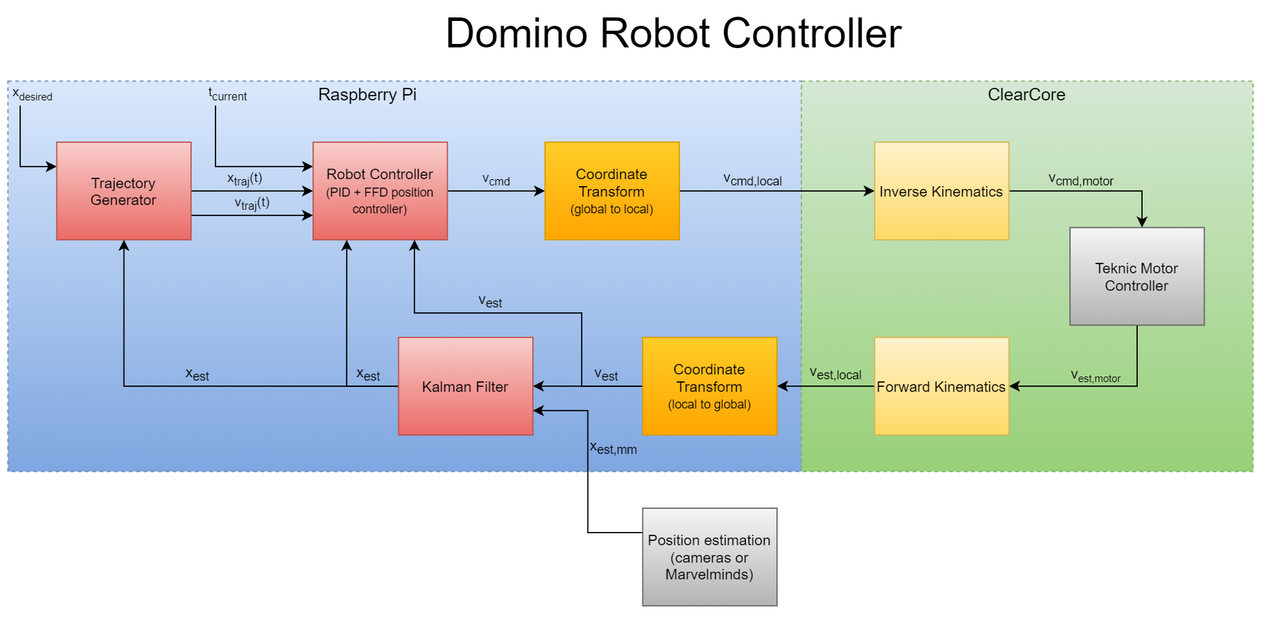
Since the Domino Robot and all its hardware and software were custom designed, this meant that I also needed to design a custom control system from the ground up. The diagram below shows all of the major components of the control system and I will explain each one in detail.
Major components of the Domino Robot Control System (click to enlarge)
Trajectory generation
The first step is to generate a trajectory for the controller to follow. I won’t go into too much detail here as I have written a whole post about the details of how this works. In summary though, the trajectory generator uses the desired position and an estimate of the current position to generate a time-parameterized trajectory which can quickly return a target position and target velocity for any time. This generation step is run once at the start of the move, and then the fast lookup step is run for every loop of the controller afterwards until the move is completed.
Robot Controller
The robot controller is responsible for taking the target position and velocity from the trajectory, comparing that with the estimated position and velocity from the feedback loop, and computing a velocity to command to the rest of the system. This uses a very standard PID controller with one slight change, which is the addition of a feedforward term. This feedforward term ensures that the commanded velocity tracks the target velocity more closely rather than waiting for some error to accumulate before commanding motion. The PID values were empirically tuned (that’s a fancy way to say trial and error ) to give good tracking performance while minimizing oscillations and overshoot.
Frame Transformation (World -> Robot)
All of the previous steps have happened with reference to the world, or global, coordinate frame. However, in order to turn the motors correctly, the commanded velocity must be transformed into the local frame of the robot. The robot coordinate frame is defined at the center of rotation of the robot with the x axis facing forwards (from the center of the robot towards the tray), the y axis facing to the left, and the z axis straight up. Since the global coordinate frame is also defined with the z axis facing up, this frame transformation can be reduced to a simple 2D rotation based on the robot’s heading. The equations look like:
\begin{align*} v^L_x =& v^G_xcos(\theta^G) + v^G_ysin(\theta^G) \\ v^L_y =& - v^G_xsin(\theta^G) + v^G_ycos(\theta^G) \\ v^L_a =& v^G_a \\ \end{align*}
where the superscripts $L$ and $G$ denote whether the value is in the local or global frames, respectively. The commanded velocity in the local robot frame is then sent to the ClearCore motor controller which handles the next steps in the control loop.
Inverse Kinematics
Once the ClearCore receives the local robot velocity, it needs to convert that into the actual wheel velocities needed. I call this step ‘Inverse Kinematics’ even though that is a little bit of a misnomer as inverse kinematics typically refers to a robot arm or manipulator, but a similar process is being performed here: namely, computing joint or wheel velocities from a commanded cartesian velocity. This is done with the following equations:
\begin{align*} v_{m0} =& -\frac{B}{R}(-\frac{1}{\sqrt{3}}v^L_x + \frac{1}{2} v^L_y + Dv^L_a) \\ v_{m1} =& -\frac{B}{R}(\frac{1}{\sqrt{3}}v^L_x + \frac{1}{2} v^L_y + Dv^L_a) \\ v_{m2} =& -\frac{B}{R}(-\frac{1}{2} v^L_y + Dv^L_a) \\ \end{align*}
where $B$ is the belt ratio between the motor and wheels, $R$ is the radius of the wheels, and $D$ is the distance from the wheel to the center of rotation.
Motor Controller
Now that the commanded motor velocities have been computed, they can be sent to the motors via the MoveVelocity command that Teknic provides on the ClearCore. The motors and underlying ClearPath software handles all of the precise tracking (and boy are they precise) so that I don’t have to worry about it. Note that the ClearPath motors do have their own velocity and acceleration limits, as well as built in smoothing, but I have ensured that the limits on the motors are higher than the limits set by the trajectory generator and the smoothing is reduced so the motors should simply be tracking the input without too much additional processing on top.
After sending the velocities to the motors, the next step in a control loop like this is typically to read an encoder or some other source to measure the actual velocity and compute the robot odometry based on that. However, with the ClearPath motors that I am using, this isn’t actually that necessary because they handle the tracking so accurately. However, due to previous versions of the robot needing this feature and it already being implemented when we switched to the ClearPath motors, I decided to continue to use an odometry feedback loop even though it probably isn’t fully necessary. The ClearPath motors I am using don’t actually have a way to directly measure the current velocity and the best I can measure is the reference velocity which is my commanded velocity after the additional ClearPath filtering/limiting (which, if things are configured correctly, should be very minimal).
Forward Kinematics
The ‘measured’ motor velocities need to be converted back into the local robot frame and this can be done by reversing the ‘Inverse Kinematic’ equations above to get:
\begin{align*} v^L_x =& -\frac{R}{3B}(-\frac{1}{\sqrt{3}}v_{m0} + \frac{1}{\sqrt{3}}v_{m1} ) \\ v^L_y =& -\frac{R}{3B}(v_{m0} + v_{m1} - 2v_{m2} ) \\ v^L_a =& -\frac{R}{3BD}(v_{m0} + v_{m1} + v_{m2} ). \\ \end{align*}
These local cartesian velocity values are then sent from the ClearCore back to the Raspberry Pi for further processing.
Frame Transformation (Robot ->World)
Similar to the transformation from the world to robot frames performed above, the reverse has to be performed on the ‘measured’ velocity to get it back into the world frame. Those equations are:
\begin{align*} v^G_x =& v^L_xcos(\theta^G) - v^L_ysin(\theta^G) \\ v^G_y =& v^L_xsin(\theta^G) + v^L_ycos(\theta^G) \\ v^G_a =& v^L_a \\ \end{align*}
Kalman filter
The last major part of the control loop is to use the ‘measured’ velocity and additional sensor input to update the estimated state of the robot for feeding back into the PID controller. This is done using a Kalman Filter. I won’t go into all the details of how the filter works here (other folks have explained it much better than I could), but the gist is that the filter can efficiently combine multiple measurement sources to produce a better estimate of the state than using just one source alone could. In this case, the prediction step of the filter is performed using the velocity in the world frame and the update step of the filter is done with a position estimate coming one of two additional sensors (more details in the next section).
Control Modes
Where this position measurement comes from depends on what mode the control system is running in. There are three main modes that are defined: MOVE_COARSE, MOVE_FINE, and MOVE_VISION. Each of these different modes has slightly different trajectory generation parameters and control gains in addition to using a different measurement source for the position estimate.
In the coarse mode, the robot drives faster, doesn’t care as much about the accuracy of the final position, and only sometimes uses updates from the Marvelmind Indoor ‘GPS’. It only uses the updates some times because the latency of the measurements makes them much less accurate when the robot is at higher speeds, so it only uses the position updates when the velocity is reasonably slow. This coarse mode is used for most driving segments away from the domino field where speed is more important than accuracy.
In the fine mode, the max speed is lower, accuracy of the final position is a little bit more important, and the position is updated much more frequently with the Marvelmind sensors which have an accuracy on the order of $\pm 2$cm. This mode is used for the final approach movement near the domino field to ensure the position is accurate enough to avoid knocking over dominos.
The final motion to line up the dominos is done with the vision mode. This mode uses the IR cameras on the robot to tracker markers on the ground which have been very precisely placed and can provide position measurements that are accurate on the order of millimeters. In this mode, the trajectory generation limits are even lower and the PID controller is tuned to ensure a very high level of accuracy.
Closing the Loop
Finally, the estimated position from the Kalman Filter as well as the estimated velocity are fed back into the PID controller so that the position and velocity error can be used to compute the next velocity command and the loop repeats.
Results
The result of this control loop is that the robot drives smoothly with the controller tracking the position and velocity very accurately. In fact, I had a hard time even finding a plot to show that was marginally interesting because most of the ones I looked at have all the lines stacked right on top of each other.
A plot of the velocities from the controller during a movement (click to enlarge). You can see how the controller works to keep the actual velocity close to the target velocity. Some of the spikes in the graph where the controller pushes the actual velocity away from the target are likely due to correcting for a position error.

The robot smoothly executing a motion.